Markov Decision Processes

INTRODUCTION

Markov decision processes (MDPs), also known as discrete-time controlled Markov processes in the control literature, are a class of discrete-time stochastic control processes with a simple structure that makes them useful in many applications. For example, in reinforcement learning it is assumed that the underlying dynamics can be modeled using MDPs. This blog post isn’t about the applications though, but rather about the more technical existence and uniqueness questions — questions which are often ignored. We will start with carefully defining the Markov decision process and then show a few intuitive results, the last of them being the famous dynamic programming equation.

In an MDP there is an underlying discrete-time Markov process whose trajectory can be influenced by a decision maker by choosing actions from a pre-specified class of admissible actions. The goal is choose actions in such a way so as to optimize a performance criterion. The state of the system at time \(n+1\) then depends, in a Markovian way, on the state of the system and the action chosen at time \(n.\) Depending on how general the state spaces and action space are, this framework can model a wide variety of interesting problems.

Let us discuss a toy problem—inventory control problem—for motivation. You are the manager of a distribution centre which sells the product to shops and buys the product in bulk from a factory. Suppose the maximum capacity of the distribution centre is \(C\) units, and therefore the state space is \(\mathsf S = [0, C],\) i.e., the state of the distribution centre at time \(n\) is a random variable \(X_n\) taking values in \(\mathsf S.\) The action that you can take is order some quantity of product from the factory. The action space \(\mathsf A\) also equals \([0,C]\). At time \(n\) you can observe the state \(X_n\) of the system, and with a policy in mind you order \(A_n\) units from the factory. Of course, \(A_n\) must take values in \([0, C-X_n]\). The demand from the shops is given by the i.i.d. random variables \(\{\xi_n\}_{n \ge 0}\) with a common distribution \(\mu\) on \(\mathsf S.\) It costs \(h\) dollars per unit of product to hold the product, \(b\) dollars per unit of product to buy the product, and earns \(s\) dollars per unit of product to sell the product. Any unmet demand is simply lost revenue. How should you choose a policy \(\pi = \{A_n\}_{n=0}^N\) to maximize the revenue over, say, \(N\) days?

Let us write the model more precisely. Suppose on day \(0\) you start with \(X_0 = x_0\) units of product, which is a constant. Then we have

\[\begin{aligned} X_{n+1} = \max\{0, X_{n}+A_{n}-\xi_{n}\} =: f(X_{n}, A_{n}, \xi_{n}), \quad 0 \le n < N.\end{aligned}\]

The revenue on day \(n\) is

\[\begin{aligned} R_n = s \min\{\xi_n, X_n\} - b A_n - h X_n, \quad 0 \le n \le N.\end{aligned}\]

The total expected revenue is

\[\begin{aligned} J_N(\pi, x_0) = \mathbb E \left[ \sum_{n=1}^N R_n \right].\end{aligned}\]

Does there exist an admissible policy \(\pi^*\) such that it maximises the total expected revenue? That is,

\[\begin{aligned} J_N(\pi^*, x_0) = \sup_{\pi} J_N(\pi, x_0).\end{aligned}\]

Is \(\pi^*\) optimal for every starting state \(x_0\)? It will be more convenient to model the transition dynamics of such a model using stochastic kernels, which informally model the transition probabilities of the process. That is, we want to find a stochastic kernel \(\kappa\) from \(\mathsf S \times \mathsf A\) to \(\mathsf S\) which gives the probability of the state at day \(n+1\) being in \(B \subseteq \mathsf S\) given that on day \(n\) the state was \(X_{n}\) and we took action \(A_n\). We can do this as follows

\[\begin{aligned} \kappa((X_n,A_n), B) = \mu(\{s \in \mathsf S : f(X_n,A_n,s) \in B\}).\end{aligned}\]

We haven’t been very precise about our formulation. To this end, let us start by defining the objects like stochastic kernels and sets which will define our action and state spaces.

SETTING THE STAGE

I had initially intended for this section to be a small one, but as I wrote I couldn’t help but go on a ramble since it helped me learn. If you are already comfortable with the notions of standard Borel spaces, stochastic kernels (also known as Markov kernels or transition probability kernels) and regular conditional distributions, or if you don’t want to be fully rigorous and are okay with understanding the core ideas without bothering too much with rigour and notation, feel free to skip directly to the section on Markov Decision Process.

Note on notation: I will be using sans serif typestyle for spaces, for example \(\mathsf{S}, \mathsf{T}, \mathsf{A}\) etc., and script typestyle for \(\sigma-\)algebras, for example, \(\mathscr{S}, \mathscr{T}, \mathscr{A}\) etc. In this section I will be fastidiously careful about writing the \(\sigma-\)algebra, but starting from the next section on Markov Decision Processes I often won’t write the \(\sigma-\)algebra explicitly because we will dealing with topological spaces and Borel \(\sigma-\)algebra is to be assumed implicit. But if I am forced to write, then I’ll use the script typestyle of a letter to denote the Borel \(\sigma-\)algebra of the space written in sans serif typestyle of the corresponding letter; for example, \(\mathscr{A}\) for \(\mathsf A.\) We denote the vector space of measurable functions from \((\mathsf X, \mathscr X)\) to \(\mathbb R\) by \(\mathscr X\) — the context will make it clear if we are referring to a function or a set, and what the domain of the function is. We denote the cone (i.e., stable under sums and multiplication by positive constants) of measurable functions from \((\mathsf X, \mathscr X)\) to \([0, +\infty]\) by \(\mathscr X_+.\)

Standard Borel Space

I discussed the notion of standard Borel spaces in the blog post on conditional probability, but since they play an important role in our discussion on Markov decision processes, let me elaborate on them a bit more here. Standard Borel spaces are usually studied under the banner of descriptive set theory and are intimately connected with other descriptive set theoretic concepts like analytic spaces, Lusin spaces and Souslin spaces. We will not focus on this side of the standard Borel spaces though, but rather on some important probabilistic results that can be formulated at this level of generality.

Generally speaking, very few meaningful statements can be made about Markov decision processes when we impose no regularity structure on the spaces involved and let them be any measurable spaces. This is where standard Borel spaces come in — powerful results can be concluded with this structure, and yet they are sufficiently general to be satisfying.

Polish Space

Let us start by recalling Polish spaces.

Definition 1 (Polish Space): A Polish space is a separable, completely metrizable topological space.

Examples

Any set with the discrete topology is completely metrizable, and therefore if it is countable it is Polish. So, for example, \(\{0,1\}\), \(\mathbb N\) and \(\Z\), each with the discrete topology, are Polish.
\(\mathbb R^n\) with the usual topology is Polish, for each \(n \in \mathbb N.\)
The topology of any (real or complex) Banach space is completely metrizable, and therefore separable Banach spaces are Polish.
The completion of a separable metric space is Polish.
Any closed subspace of a Polish space is Polish.
The disjoint union of countably many Polish spaces is Polish.
The product of countably many Polish spaces is Polish.

All of these examples follow from elementary properties of metric spaces. So, for example, to show the last example, first show that the product of countably many separable metric spaces is itself separable using the definition of product topology, and then show that the product of countably many complete metric spaces is itself a complete metric space using the idea of the product metric and the definition of Cauchy sequences.

Polish spaces are the probabilist’s favourite spaces to work with since they are simple to deal with and a lot of spaces are Polish, while almost all results that hold in \(\mathbb R\) still hold in a Polish space. For example, if \((\mathsf X,d_{\mathsf X})\) is a compact metric space and \((\mathsf Y, d_{\mathsf Y})\) is Polish, then \(C(\mathsf X,\mathsf Y)\), the set of continuous functions from \(\mathsf X\) to \(\mathsf Y\) with the uniform metric \(d(f,g) = \sup_{x \in \mathsf X} d_{\mathsf Y}(f(x), g(y))\), is Polish.

Standard Borel Space

Recall the notion of isomorphism between algebraic objects or the notion of homeomorphism between topological spaces. Both these notions give a bijective correspondence between two objects that preserves the algebraic or the topological structure. In a similar spirit we have the notion of isomorphism between two measurable spaces.

Definition 2 (Isomorphism and Borel isomorphism): Two measurable spaces \((\mathsf S, \mathscr{S})\) and \((\mathsf T, \mathscr{T})\) are called isomorphic iff there is a bijective function \(f \colon \mathsf S \to \mathsf T\) such that both \(f\) and its inverse \(f^{-1}\) are measurable. The function \(f\) is called an isomorphism. In the special case where \(\mathsf S\) and \(\mathsf T\) are topological spaces equipped with their Borel \(\sigma-\)algebras and \(f \colon \mathsf S \to \mathsf T\) is an isomorphism, \(f\) is called a Borel isomorphism, and \(\mathsf S\) and \(\mathsf T\) are called Borel isomorphic.

Definition 3 (Standard Borel space): A standard Borel space is a measurable space isomorphic to a Polish space endowed with its Borel \(\sigma-\)algebra.

Let me list some properties about standard Borel spaces without proof–mostly to justify using them as our default spaces.

Proposition 1: The product of countably many standard Borel spaces is a standard Borel space.

Proposition 2: A measurable subset \(\mathsf S\) of a standard Borel space \((\mathsf T, \mathscr T)\), where we endow \(\mathsf S\) with the \(\sigma-\)algebra \(\mathscr S = \{ T \cap \mathsf S \,: \, T \in \mathscr T\}\), is a standard Borel space. For the other direction, if \(\mathsf S\) is a metrizable topological space endowed with its Borel \(\sigma-\)algebra \(\mathscr S\), then \((\mathsf S, \mathscr S)\) is a standard Borel space if and only if \(\mathsf S\) is homeomorphic to a Borel subset of a Polish space.

It is obvious from the definition that two countable metrizable spaces are Borel isomorphic if and only if they have the same cardinality. For the uncountable case, it is not immediately obvious when two spaces are Borel isomorphic. The next proposition is a deep and surprising result.

Proposition 3: All uncountable standard Borel spaces are mutually isomorphic.

Observe that \([0,1]\) endowed with its Borel \(\sigma-\)algebra is a Polish space, and therefore every uncountable standard Borel space is isomorphic to \(([0,1], \mathscr{B}([0,1])),\) where the notation \(\mathscr B(\mathsf T)\) denotes the Borel \(\sigma-\)algebra of a topological space \(\mathsf T.\) This observation will prove to be very helpful in proving existence result for regular conditional distributions, in proving the disintegration theorem etc.

Proposition 4: If a bijective map between standard Borel spaces is measurable, then the inverse map is also measurable.

This, in particular, implies that if both \((\mathsf S, \mathscr S_1)\) and \((\mathsf S, \mathscr S_2)\) are standard Borel spaces, then \(\mathscr S_1 = \mathscr S_2.\) Now recall that the Borel \(\sigma-\)algebra on \([0,1]\) is a strict subset of the Lebesgue \(\sigma-\)algebra on it. This gives us a simple example of a measurable space which is not a standard Borel space.

A very useful result that further justifies the case for using standard Borel spaces is the following: Let \((\mathsf S, \mathscr S)\) be a standard Borel space and let \(\mathcal{P}(\mathsf S)\) denote the collection of all probability measures on \((\mathsf S, \mathscr S).\) Endow \(\mathcal{P}(\mathsf S)\) with the topology of weak convergence, i.e., the topology generated by the evaluation maps \(\mathcal{P}(\mathsf S) \ni\mu \mapsto \mu(S) \in [0,1]\), where \(S\) varies over \(\mathscr S\) (or equivalently, by the maps \(\mu \mapsto \int f \, \mathrm{d}\mu\), where \(f\) varies over \(C_b(\mathsf S)\)). Then \(\mathcal{P}(\mathsf S)\) equipped with its Borel \(\sigma-\)algebra is a standard Borel space. This fact becomes useful when dealing with partially observable MDPs. Here a standard approach is to transform them into an equivalent “completely observable” MDP (the one in Definition 14 ahead) with a larger state space, a space of probability measures.

A cool fact, which has no bearing on our discussion ahead, is the following.

Proposition 5: If \((\mathsf X, \mathscr X)\) and \((\mathsf Y, \mathscr Y)\) are two standard Borel spaces, then the map \(f \colon \mathsf X \to \mathsf Y\) is measurable if and only if its graph \(\llbracket f \rrbracket := \{(x, f(x)) \,:\, x \in \mathsf X\}\) is a measurable subset of the product space \((\mathsf X \times \mathsf Y, \mathscr X \otimes \mathscr Y).\)

Stochastic Kernels

Suppose that a particle is moving randomly in a state space given by a measurable space \((\mathsf S, \mathscr{S})\). We would like to be able to know the probability, denoted with say \(\kappa(x, B)\), of the particle finding itself in a set \(B \in \mathscr{S}\) after a unit of time given that it started at state \(x \in \mathsf S.\) Stochastic kernels model this notion of transition probabilities in a natural manner and we will rely heavily on them in our discussion.

Definition 4 (Stochastic kernel): Let \((\mathsf S, \mathscr{S})\) and \((\mathsf T, \mathscr{T})\) be two measurable spaces. A map

\[ \kappa \colon \mathsf S \times \mathscr{T} \to [0,1] \]

is called a stochastic kernel or a Markov kernel or a transition probability kernel from \((\mathsf S, \mathscr{S})\) to \((\mathsf T, \mathscr{T})\)–or, briefly, from \(\mathsf S\) to \(\mathsf T\)–if

\(x \mapsto \kappa(x, B)\) is \(\mathscr{S}-\)measurable for each \(B \in \mathscr{T}\), and
\(B \mapsto \kappa(x,B)\) is a probability measure on \((\mathsf T, \mathscr{T})\) for each \(x \in \mathsf S.\)

We often denote \(\kappa(x, B)\) with \(\kappa_x(B)\) and the mapping \(x \mapsto \kappa(x, B)\) with \(\kappa(B).\) If \((\mathsf T, \mathscr{T}) = (\mathsf S, \mathscr{S})\), we simply say a kernel on \((\mathsf S, \mathscr{S})\) or, even more simply, on \(\mathsf S\). Instead of saying a stochastic kernel from \((\mathsf S, \mathscr{S})\) to \((\mathsf T, \mathscr{T}),\) some books and papers say a stochastic kernel on \((\mathsf T, \mathscr{T})\) given \((\mathsf S, \mathscr{S}).\) We can view the stochastic kernel \(\kappa\) as a measurable function from \(\mathsf S\) to the space \(\mathcal{P}(\mathsf T)\) of probability measures on \((\mathsf T, \mathscr{T})\), where the \(\sigma-\)algebra on \(\mathcal{P}(\mathsf T)\) is generated by the weak topology, as mentioned above. For this reason, stochastic kernel are also called random probability measures. We can also view the stochastic kernel \(\kappa\) as a probabilistic generalization of the concept of function from \(\mathsf S\) to \(\mathsf T\)–instead of associating with each \(x \in \mathsf S\) a unique value from \(\mathsf T\), we associate a probability distribution on \(\mathsf T.\)

The term kernel, without the adjective stochastic, will be used to denote a similar object as a stochastic kernel except that the property 2 in the definition above states \(B \mapsto \kappa(x,B)\) is a measure on \((\mathsf T, \mathscr{T})\) for each \(x \in \mathsf S.\)

Examples

Given a measurable space \((\mathsf S, \mathscr{S})\), the function
\[\begin{aligned} \mathsf S \times \mathscr{S} \ni (x,B) \mapsto \kappa(x,B) = \begin{cases} 1 &\text{if } x \in B, \\ 0 &\text{if } x \in \mathsf S \setminus B \end{cases}\end{aligned}\]
defines a stochastic kernel on \((\mathsf S, \mathscr{S})\), called the unit kernel. For each \(x \in \mathsf S\), the measure \(B \mapsto \kappa(x,B)\) is the Dirac measure \(\delta_x\) on \((\mathsf S, \mathscr{S})\) at \(x.\)
Given two measurable spaces \((\mathsf S, \mathscr{S})\) and \((\mathsf T, \mathscr{T})\) and a measure \(\nu\) on \((\mathsf T, \mathscr{T})\), the function
\[\begin{aligned} \mathsf S \times \mathscr{T} \ni (x,B) \mapsto \kappa(x, B) := \nu(B)\end{aligned}\]
defines a kernel from \((\mathsf S, \mathscr{S})\) to \((\mathsf T, \mathscr{T})\) which does not depend on \(x.\) Therefore, every measure can be seen as a special type of a kernel.
Given two measurable spaces \((\mathsf S, \mathscr{S})\) and \((\mathsf T, \mathscr{T})\) and a measurable function \(f \colon \mathsf{S} \to \mathsf T\), the function
\[\begin{aligned} \mathsf S \times \mathscr T \ni (x,B) \mapsto \kappa(x,B) := \mathbf{1}_B(f(x))\end{aligned}\]
defines a stochastic kernel from \((\mathsf S, \mathscr{S})\) to \((\mathsf T, \mathscr{T}).\)
Consider the two measurable spaces \((\mathsf S = \{1, 2, \ldots, n\}, \mathfrak{P}(\mathsf S))\) and \((\mathsf T = \{1, 2, \ldots, m\}, \mathfrak{P}(\mathsf T))\) for two positive integers \(n\) and \(m\), with \(\mathfrak{P}(\mathsf X)\) denoting the power set of a set \(\mathsf X.\) Suppose we are given an \(n \times m\) matrix \(\mathbf K\) containing non-negative elements such that the sum along each row is \(1.\) Then the function \(\kappa\) defined by
\[\begin{aligned} \mathsf S \times \mathfrak{P}(\mathsf T) \ni (i,B) \mapsto \kappa(i, B) := \sum_{j \in B} \mathbf K_{i,j}\end{aligned}\]
is a stochastic kernel from \(\mathsf S\) to \(\mathsf T.\) The case where \(\mathsf S\) or \(\mathsf T\) are countably infinite is similar.

Regular Conditional Distribution

In most discussions of MDPs the notion of conditional distribution and the associated notation are left frustratingly ambiguous. To remedy this let us spend some time discussing regular conditional distribution and disintegration in this subsection and the next. I also discussed the idea of regular conditional distribution in a previous blog post.

Let us start with a well-known but important result.

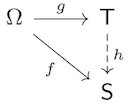
Lemma 1 [Doob-Dynkin factorization lemma]: Let \((\Omega, \mathscr{F})\) and \((\mathsf T, \mathscr T)\) be arbitrary measurable spaces, and \((\mathsf S, \mathscr S)\) be a standard Borel space endowed with its Borel \(\sigma-\)algebra. Let \(f \colon \Omega \to \mathsf S\) and \(g \colon \Omega \to \mathsf T\) be measurable functions. Then \(f\) is \(\sigma(g)-\)measurable if and only if \(f = h \circ g\) for some measurable function \(h \colon \mathsf T \to \mathsf S.\)

The sufficiency is very easy to verify. Indeed, if \(f = h \circ g\) for some measurable function \(h \colon \mathsf T \to \mathsf S,\) then for any \(S \in \mathscr S\) we have \(f^{-1}(S) = g^{-1}(h^{-1}(S)) \in \sigma(g).\)

For the necessity, we first prove the lemma for the case \(\mathsf S = [0,1].\) Then using Propositions 2 and 3 we will extend the argument to an arbitrary standard Borel space. This is the typical way to deal with standard Borel spaces.

So suppose that \(\mathsf S = [0,1].\) If \(f = \mathbf{1}_A\) for \(A \in \sigma(g),\) then by the definition of \(\sigma(g)\) there exists a set \(B \in \mathscr{T}\) such that \(A = g^{-1}(B).\) Then we can write \(f = \mathbf{1}_B \circ g,\) where \(\mathbf{1}_B \colon \mathsf T \to \mathsf S\) is of course measurable. Linearity allows us to deduce our desired conclusion for the case when \(f\) is a simple function. For a general \(\sigma(g)-\)measurable \(f,\) we know that we can find a sequence \(\{f_n\}\) of nonnegative simple \(\sigma(g)-\)measurable functions with \(f_n \uparrow f.\) Therefore, for each \(n\) we may choose measurable \(h_n \colon \mathsf T \to \mathsf S\) such that \(f_n = h_n \circ g.\) Then \(h := \sup_n h_n\) is again measurable, and we have

\[\begin{aligned} f = \sup_n f_n = \sup_n (h_n \circ g) = \left(\sup_n h_n\right) \circ g = h \circ g.\end{aligned}\]

Finally, we extend the proof to the general case of \(\mathsf S\) being a standard Borel space. Propositions 2 and 3 imply that there exists an isomorphism \(\iota \colon \mathsf S \to [0,1].\) The preceding argument applied to the \(\sigma(g)-\)measurable function \(\iota \circ f \colon \Omega \to [0,1]\) implies that there exists a measurable function \(h_\iota \colon \mathsf T \to [0,1]\) such that \(\iota \circ f = h_\iota \circ g.\) But since \(\iota\) is a bijection, we can write \(f = (\iota^{-1} \circ h_\iota) \circ g.\) The function \(h := \iota^{-1} \circ h_\iota \colon \mathsf T \to \mathsf S\) is our desired measurable function.

Under the setting of the above lemma, suppose \(X \colon \Omega \to [0, \infty]\) is a random variable and \(Y \colon \Omega \to \mathsf T\) is a measurable function. Then the lemma above implies that the conditional expectation \(\mathbb{E}[X \mid Y]\) can be written as \(h \circ Y\) for some measurable \(h \colon \mathsf T \to [0, \infty].\)

Notation: We use \(\mathbb{E}[X \mid Y=y]\) to denote \(h(y).\)

Here the non-negativity of \(X\) is inessential, except for ensuring that the conditional expectation exists—we could have assumed \(X\) to be real-valued and integrable.

Before we discuss regular conditional distribution in full generality, let us discuss the simpler concept of regular conditional probability.

Regular Conditional Probability

Let \((\Omega, \mathscr{F}, \mathbb P)\) be a probability space and \(\mathscr G\) be a sub-\(\sigma\)-algebra of \(\mathscr F.\) For \(A \in \mathscr F,\) if we denote with \(\kappa(A)\) a version of the conditional probability \(\mathbb{P}(A \mid \mathscr G),\) and use \(\kappa_\omega(A)\) to denote \(\kappa(A)(\omega),\) then we have

\(\kappa(\varnothing) = 0\) a.s.;
\(\kappa(\Omega) = 1\) a.s.;
the mapping \(\omega \mapsto \kappa_\omega(A)\) is \(\mathscr G-\)measurable for each \(A \in \mathscr F\); and
by the monotone convergence theorem for conditional expectations, for every disjointed sequence \(\{A_n\}\) in \(\mathscr F,\)
\[\begin{aligned} \kappa_\omega\left( \bigcup_n A_n \right) = \sum_n \kappa_\omega(A_n)\end{aligned}\]
for every \(\omega\) outside a null set.

With these properties the function \((\omega, A) \mapsto \kappa_\omega(A)\) looks very much like a stochastic kernel. But the fact that the null set in property 4 depends on the sequence \(\{A_n\}\) and that there could be uncountably many such sequences, means that \(\kappa\) is, in general, not a stochastic kernel. When \(\kappa\) can be made into a stochastic kernel we get a very special object called a regular version of the conditional probability, or simply regular conditional probability.

Definition 5 (Regular conditional probability): Let \((\Omega, \mathscr{F}, \mathbb P)\) be a probability space and \(\mathscr G\) be a sub-\(\sigma\)-algebra of \(\mathscr F.\) For \(A \in \mathscr F\) let \(\kappa(A)\) be a version of the conditional probability \(\mathbb{P}(A \mid \mathscr G).\) Then \(\Omega \times \mathscr F \ni (\omega, A) \mapsto \kappa_\omega(A) \in [0,1]\) is said to be a regular version of the conditional probability \(\mathbb{P}(\cdot \mid \mathscr G)\) if it is a stochastic kernel from \((\Omega , \mathscr G)\) to \((\Omega, \mathscr F).\)

Recall Theorem 2 from a previous blog post which I state here again:

Proposition 6: Under the setting of Definition 5, if \(X\) is a real-valued random variable whose expectation exists, then

\[\begin{aligned} \omega \mapsto \int_\Omega X \, \mathrm{d}\kappa_\omega\end{aligned}\]

is a version of the conditional expectation \(\mathbb{E}\left[ X \mid \mathscr G \right].\)

When does a regular conditional probability exist? Intuitively, we need to impose conditions on either the sub-\(\sigma\)-algebra \(\mathscr G\) or on the probability space \((\Omega, \mathscr{F}, \mathbb P).\) In the first case, suppose \(\mathscr G\) is generated by a countable partition \(\{A_n\}\) of \(\Omega,\) which is the case when \(\mathscr G\) is generated by a random variable taking values in a countable space. Then define

\[\begin{aligned} \kappa_\omega(A) = \sum_n \mathbb{P}_{A_n}(A) \;\mathbf{1}_{A_n}(\omega), \quad \omega \in \Omega, \, A \in \mathscr F,\end{aligned}\]

where \(\mathbb{P}_B(A)\) is defined to be any number in \([0,1]\) satisfying \(\mathbb{P}(A \cap B) = \mathbb{P}(B)\, \mathbb{P}_B(A).\) This makes \(\kappa\) a regular conditional probability because \(A \mapsto \mathbb{P}_B(A)\) is a probability measure.

For the case where \(\mathscr{G}\) could be arbitrary, we have the following result.

Theorem 1: If \((\Omega, \mathscr{F})\) is a standard Borel space, then a regular version of the conditional probability \(\mathbb{P}(\cdot \mid \mathscr G)\) as in Definition 5 exists.

The proof of this theorem will be a simple consequence of the existence of regular conditional distributions which we discuss next.

Regular Conditional Distribution

Definition 6 (Regular conditional distribution): Let \((\Omega, \mathscr{F}, \mathbb P)\) be a probability space, \(\mathscr G\) be a sub-\(\sigma\)-algebra of \(\mathscr F,\) \((\mathsf S, \mathscr S)\) be a measurable space, and \(X \colon \Omega \to \mathsf S\) be a random element. The regular conditional distribution of \(X\) given \(\mathscr G\), or simply, conditional distribution of \(X\) given \(\mathscr G\) is any stochastic kernel \(\kappa\) from \((\Omega, \mathscr G)\) to \((\mathsf S, \mathscr S)\) such that \[\begin{aligned} \kappa(B) = \mathbb{P}(\{X \in B\} \mid \mathscr G) \text{ a.s.}, \quad B \in \mathscr S.\end{aligned}\]

Theorem 2: Under the setting of Definition 6, if \((\mathsf S, \mathscr S)\) is a standard Borel space, then there exists a version of the regular conditional distribution of \(X\) given \(\mathscr G.\)

(From (Cinlar, 2011) Theorem IV.2.10) As in the proof of Lemma 1, we first give the proof for a special case of \(\mathsf S\), which here we assume \(\mathsf S = \overline{\mathbb R} := [-\infty, +\infty]\) and \(\mathscr S\) being its Borel \(\sigma-\)algebra. For each \(q \in \mathbb{Q},\) define

\[\begin{aligned} C_q := \mathbb{P}(\{X \le q\} \mid \mathscr G).\end{aligned}\]

We shall construct the regular conditional distribution \(\kappa\) of \(X\) given \(\mathscr G\) from these countably many random variables \(\{C_q\}_{q \in \mathbb Q}.\) For \(q < r,\) we have \(\{X \le q \} \subseteq \{X \le r\},\) and therefore by the monotonicity of conditional expectations the event

\[\begin{aligned} \Omega_{qr} = \{C_q \le C_r\}\end{aligned}\]

is an almost sure event and is in \(\mathscr G.\) Then the countable intersection

\[\begin{aligned} \Omega_0 = \bigcap_{\stackrel{q,r \in \mathbb Q}{q < r}} \Omega_{qr}\end{aligned}\]

is also an almost sure event and is in \(\mathscr G.\) Fix an arbitrary \(\omega_0 \in \Omega_0.\) Then the mapping

\[\begin{aligned} \mathbb{Q} \ni q \mapsto C_q(\omega_0) \in [0,1]\end{aligned}\]

is non-decreasing, and thus, for each \(t \in \mathbb R,\) we can define

\[\begin{aligned} C_t(\omega_0) = \lim_{\stackrel{q \in \mathbb Q}{q > t}} C_q(\omega_0).\end{aligned}\]

The resulting extension \(\mathbb{R} \ni t \mapsto C_t(\omega_0) \in [0,1]\) is non-decreasing, right-continuous, and satisfies \(\lim_{t \to -\infty} C_t(\omega_0) = 0\) and \(\lim_{t \to \infty} C_t(\omega_0) = 1,\) and therefore is a probability distribution function. Denote with \(\overline{\kappa}_{\omega_0}\) the probability measure on \(\mathscr S\) associated with this probability distribution function. Now define

\[\begin{aligned} \kappa_\omega(B) := \mathbf{1}_{\Omega_0}(\omega) \;\overline{\kappa}_\omega(B) + \mathbf{1}_{\Omega \setminus \Omega_0}(\omega) \; \delta_0(B), \quad \omega \in \Omega, B \in \mathscr S.\end{aligned}\]

We claim that \(\kappa\) is a regular conditional distribution of \(X\) given \(\mathscr G.\) Let us verify the required properties one by one—the first two being the two properties in Definition 4 and the last being (1).

We will use Dynkin’s theorem (Theorem 4 here), which is a type of monotone class argument. Consider the collection
\[\begin{aligned} \mathscr D = \left\{B \in \mathscr S \; : \; \omega \mapsto \kappa_\omega(B) \text{ is } \mathscr G\text{-measurable}\right\}.\end{aligned}\]

\(\kappa_\omega(\mathsf S) = 1\) for all \(\omega \in \Omega\) and therefore \(\omega \mapsto \kappa_\omega(\mathsf S)\) is \(\mathscr G-\)measurable, showing \(\mathsf S \in \mathscr D.\) For \(A \subseteq B\) with \(A, B \in \mathscr S,\) we have \(\kappa_\omega(B \setminus A) = \kappa_\omega(B) - \kappa_\omega(A),\) and therefore if \(A\) and \(B\) are in \(\mathscr D\) with \(A \subseteq B\) then so does \(B \setminus A.\) Finally, if \(B_1 \subseteq B_2 \subseteq \cdots\) is an increasing sequence in \(\mathscr D,\) then using the continuity of measure from below and the fact that the pointwise limit of measurable functions is again measurable, we get that \(\bigcup_n B_n \in \mathscr D.\) We conclude that \(\mathscr D\) is a d-system.

By the Dynkin’s theorem, to show that \(\mathscr D = \mathscr S,\) it is enough to show that \(\mathscr D\) contains the \(\pi\)-system \(\left\{ \lbrack - \infty, t \rbrack \,:\, t \in \overline{\mathbb R}\right\}.\) For \(t = +\infty\) we have already shown that \([-\infty, t] \in \mathscr D.\) Similarly it is easy to see that for \(t = -\infty\) we have \([-\infty, t] = \varnothing \in \mathscr D.\) Fix a \(t \in \mathbb R\) and note that we can write
\[\begin{aligned} \kappa_\omega([-\infty, t]) &= \mathbf{1}_{\Omega_0}(\omega) \; C_t(\omega) + \mathbf{1}_{\Omega \setminus \Omega_0}(\omega) \; \delta_0([-\infty, t]) = \lim_{\stackrel{q \in \mathbb Q}{q > t}} \mathbf{1}_{\Omega_0}(\omega) \; C_q(\omega) + \mathbf{1}_{\Omega \setminus \Omega_0}(\omega) \; \delta_0([-\infty, t]). \end{aligned}\]

Since each of \(\left\{ C_q,\, q \in \mathbb Q\right\}, \mathbf{1}_{\Omega_0}\) and \(\mathbf{1}_{\Omega \setminus \Omega_0}\) is \(\mathscr G-\)measurable, and \(\delta_0([-\infty, t])\) is a constant, the map \(\omega \mapsto \kappa_\omega([-\infty, t])\) is \(\mathscr G-\)measurable.

We conclude that \(\omega \mapsto \kappa_\omega(B)\) is \(\mathscr G-\)measurable for each \(B \in \mathscr S.\)
For each \(\omega \in \Omega,\) \(B \mapsto \kappa_\omega(B)\) is clearly a probability measure on \(\mathscr S.\)
To verify (1), we need to show that \[\begin{aligned} \int_G \kappa(B) \, \mathrm{d}\mathbb{P} = \mathbb{P}(G \cap \{X \in B\}), \quad G \in \mathscr{G}, B \in \mathscr S.\end{aligned}\] By the same Dynkin’s theorem-type argument as in 1. above, we need to show (2) for \(B = [-\infty, t]\) with \(t \in \mathbb R.\) By the definition of \(C_q\) we get
\[\begin{aligned} \mathbb{P}(G \cap \{X \in B\}) = \mathbb{P}(G \cap \{X \le t\}) = \lim_{\stackrel{q \in \mathbb Q}{q > t}} \mathbb{P}(G \cap \{X \le q\}) = \lim_{\stackrel{q \in \mathbb Q}{q > t}} \int_G C_q \, \mathrm{d}\mathbb{P}.\end{aligned}\]
Now note that for \(\omega \in \Omega_0,\) \(C_q(\omega) \to C_t(\omega) = \kappa_\omega(B)\) as \(q \downarrow t.\) Therefore using monotone convergence theorem and the fact that \(\Omega_0\) is of full measure, we can write
\[\begin{aligned} \lim_{\stackrel{q \in \mathbb Q}{q > t}} \int_G C_q \, \mathrm{d}\mathbb{P} = \lim_{\stackrel{q \in \mathbb Q}{q > t}} \int_{G \cap \Omega_0} C_q \, \mathrm{d}\mathbb{P} = \int_G \kappa(B) \, \mathrm{d}\mathbb{P}.\end{aligned}\]
This implies (2).

This completes the proof for the special case when \(\mathsf S = \overline{\mathbb R}.\) To extend the proof to arbitrary standard Borel spaces, suppose \(\iota \colon \mathsf S \to [0,1]\) is an isomorphism. The preceding argument applied to the real-valued random variable \(\iota \circ X\) shows the existence of the regular conditional distribution \(\kappa^\iota\) of \(\iota \circ X\) given \(\mathscr G.\) Now define

\[\begin{aligned} \kappa_\omega(B) = \kappa^\iota_\omega(\iota(B)), \quad \omega \in \Omega,\, B \in \mathscr S.\end{aligned}\]

Here \(\iota(B)\) is the image of \(B\) under \(\iota.\) It is easy to check that \(\kappa\) is a stochastic kernel from \((\Omega, \mathscr G)\) to \((\mathsf S, \mathscr S).\) To verify property (1) observe that, for \(G \in \mathscr G\) and \(B \in \mathscr S,\)

\[\begin{aligned} \mathbb{P}(G \cap \{X \in B\}) = \mathbb{P}(G \cap \{\iota \circ X \in \iota(B)\}) = \int_G \kappa^\iota(\iota(B)) \, \mathrm{d}\mathbb{P} = \int_G \kappa(B) \, \mathrm{d}\mathbb{P}.\end{aligned}\]

Regular conditional probabilities and regular conditional distributions are closely related. If \(\kappa\) is a regular version of the conditional probability \(\mathbb{P}(\cdot \mid \mathscr G),\) then \(\kappa^X\) defined as

\[\begin{aligned} \kappa_\omega^X(B) := \kappa_\omega(\{X \in B\})\end{aligned}\]

is easily seen to be a regular conditional distribution of \(X\) given \(\mathscr G.\) On the other hand, Theorem 1 follows from Theorem 2. Suppose that \((\Omega, \mathscr F)\) is a standard Borel space and let \((\mathsf S, \mathscr S) = (\Omega, \mathscr F).\) Define \(X(\omega) = \omega\) for all \(\omega \in \Omega.\) Then Theorem 2 gives a regular conditional distribution \(\kappa\) of \(X\) given \(\mathscr G\) which is precisely a regular version of the conditional probability \(\mathbb{P}(\cdot \mid \mathscr G).\)

Suppose in the setting of Definition 6, we also have a measurable space \((\mathsf T, \mathscr T)\) and a random element \(Y \colon \Omega \to \mathsf T.\) Then by the conditional distribution of \(X\) given \(Y\) we will mean the conditional distribution of \(X\) given \(\sigma(Y).\)

Disintegration

Let us first recall the construction of measures on a product space, which is closely tied with disintegrations. Suppose \((\mathsf S, \mathscr{S})\) and \((\mathsf T, \mathscr{T})\) are measurable spaces, \(\mu\) is a measure on \((\mathsf S, \mathscr{S})\), and \(\kappa\) is a kernel from \((\mathsf S, \mathscr{S})\) to \((\mathsf T, \mathscr{T})\) that can be written as \(\kappa = \sum_{n=1}^\infty \kappa_n\) for kernels \(\kappa_n\) from \((\mathsf S, \mathscr{S})\) to \((\mathsf T, \mathscr{T})\) that satisfy \(\kappa_n(x, \mathsf{T}) < \infty\) for each \(x \in \mathsf{S}\) (such kernels \(\kappa\) are called \(\Sigma-\)finite). If \(f \colon \mathsf{S} \times \mathsf{T} \to [-\infty, +\infty]\) is measurable, recall that \(x \mapsto f(x,y)\) is measurable for each \(y \in \mathsf T\) and \(y \mapsto f(x,y)\) is measurable for each \(x \in \mathsf S.\) If \(f \in (\mathscr S \otimes \mathscr T)_+\), then

\[\begin{aligned} \mathsf S \ni x \mapsto \kappa f(x) := \int_{\mathsf T} f(x,y) \, \kappa(x, \mathrm{d}y) \in [0, +\infty]\end{aligned}\]

defines a non-negative measurable function. The iterated integral \[\begin{aligned} \gamma f \equiv \int_{\mathsf S \times \mathsf T} f \, \mathrm{d}\gamma := \int_{\mathsf S} \left( \int_{\mathsf T} f(x,y) \, \kappa(x, \mathrm{d}y)\right)\,\mu(\mathrm{d}x)\end{aligned}\] for \(f \in (\mathscr S \otimes \mathscr T)_+\) defines a measure \(\gamma\) on the product space \((\mathsf{S} \times \mathsf T, \mathscr S \otimes \mathscr T).\) Moreover, if \(\mu\) is \(\sigma-\)finite and \(\kappa\) is \(\sigma-\)bounded (i.e., there exists a measurable partition \(\{\mathsf T_n\}\) of \(\mathsf T\) such that \(x \mapsto \kappa(x, \mathsf T_n)\) is bounded for each \(n\)), then \(\gamma\) is \(\sigma-\)finite and is the unique measure on the product space satisfying

\[\begin{aligned} \gamma(A \times B) = \int_A\kappa(x,B) \, \mu(\mathrm{d} x), \quad A \in \mathscr{S}, B \in \mathscr{T}.\end{aligned}\]

We denote \(\gamma\) with \(\mu \otimes \kappa.\) For the special case when \(\kappa(x,B) = \nu(B)\) for some measure \(\nu\) on \(\mathscr T\), like in the example above, we denote \(\gamma\) with \(\mu \otimes \nu.\) In this special case we can interchange the order of integrals, i.e.,

\[\begin{aligned} \int_{\mathsf S} \left( \int_{\mathsf T} f(x,y) \, \nu( \mathrm{d}y)\right)\,\mu(\mathrm{d}x) = \int_{\mathsf T} \left( \int_{\mathsf S} f(x,y) \, \mu( \mathrm{d}x)\right)\,\nu(\mathrm{d}y),\end{aligned}\]

for \(f \in (\mathscr S \otimes \mathscr T)_+\) (this is known as the Tonelli’s theorem). Also if \(f \colon \mathsf{S} \times \mathsf{T} \to [-\infty, +\infty]\) is \(\mu \otimes \nu-\)integrable, then \(x \mapsto f(x,y)\) is \(\mu-\)integrable for \(\nu-\)a.e. \(y\), and \(y \mapsto f(x,y)\) is \(\nu-\)integrable for \(\mu-\)a.e. \(x\), and the interchange above holds again (this is known as the Fubini’s theorem).

Disintegration asks the converse to the construction of measures on product spaces: Given a measure \(\gamma\) on the product space \((\mathsf{S} \times \mathsf T, \mathscr S \otimes \mathscr T)\) does there exist a measure \(\mu\) on \((\mathsf S, \mathscr{S})\) and a kernel \(\kappa\) from \((\mathsf S, \mathscr{S})\) to \((\mathsf T, \mathscr{T})\) such that (3) holds? We will answer this in the affirmative for the special case for probability measures and stochastic kernels. For a more thorough discussion see the paper (Chang and Pollard, 1997).

Theorem 3 (Disintegration): Suppose \((\mathsf S, \mathscr{S})\) and \((\mathsf T, \mathscr{T})\) are measurable spaces with \((\mathsf T, \mathscr T)\) being a standard Borel space endowed with its Borel \(\sigma-\)algebra, and \(\gamma\) is a probability measure on the product space \((\mathsf{S} \times \mathsf T, \mathscr S \otimes \mathscr T).\) Then there exists a probability measure \(\mu\) on \((\mathsf S, \mathscr{S})\) and a stochastic kernel \(\kappa\) from \((\mathsf S, \mathscr{S})\) to \((\mathsf T, \mathscr{T})\) such that (3) holds for all \(f \in (\mathscr S \otimes \mathscr T)_+.\)

(From (Cinlar, 2011) Theorem IV.2.18)

We will use Theorem 2 by converting the theorem above to its special case. Define the probability space \((\Omega, \mathscr F, \mathbb P) = (\mathsf{S} \times \mathsf T, \mathscr S \otimes \mathscr T, \gamma).\) Define the random elements \(Y \colon \Omega \to \mathsf S\) and \(X \colon \Omega \to \mathsf T\) as the projections \((s,t) \mapsto s\) and \((s,t) \mapsto t\) respectively. Let \(\mu\) be the distribution of \(Y\), i.e., \(\mu(A) = \gamma(A \times \mathsf T)\) for every \(A \in \mathscr S.\) Applying Theorem 2 to \(\mathscr G = \sigma(Y)\) shows that there exists a version of the regular conditional distribution of \(X\) given \(\mathscr G,\) which we will denote by \(\overline\kappa.\) Recall that \(\overline\kappa\) is a stochastic kernel from \((\Omega, \mathscr G)\) to \((\mathsf T, \mathscr T)\) such that

\[\begin{aligned} \mathbb{E}\left[ g\,\overline\kappa(B)\right] = \mathbb{E}\left[\mathbf{1}_{\{X \in B\}} g\right], \quad B \in \mathscr T, \, g \in \mathscr G_+.\end{aligned}\]

By the structure of \(Y\), we see that \(\mathscr G\) consists of measurable rectangles of the form \(A \times \mathsf T\) for \(A \in \mathscr S.\) Therefore, the Doob-Dynkin factorization lemma implies that a function \(g \colon \Omega \to [0, \infty]\) is \(\mathscr G-\)measurable if and only if \(g((s,t)) = \overline{g}(s)\) for some measurable \(\overline{g} \colon \mathsf S \to [0, \infty].\) Now using equation (4), we conclude that \(\overline \kappa((s,t), B) = \kappa(s, B)\) for some stochastic kernel \(\kappa\) from \((\mathsf S, \mathscr S)\) to \((\mathsf T, \mathscr T).\)

If \(A \in \mathscr S\) and \(B \in \mathscr T\), equation (4) allows to write

\[\begin{aligned} \gamma(A \times B) = \mathbb{E}\left[\mathbf{1}_{\{Y \in A\}} \mathbf{1}_{\{X \in B\}}\right] = \mathbb{E}\left[\mathbf{1}_{\{Y \in A\}}\kappa(B)\right] = \int_{\mathsf S} \mathbf{1}_A(s) \kappa(s,B) \,\mu(\mathrm{d}s)\end{aligned}\]

which is equation (3) for \(f = \mathbf{1}_{A \times B}.\) Finally, a monotone class argument proves (3) for all \(f \in (\mathscr S \otimes \mathscr T)_+.\)

Now a natural question is if \(\mu\) is a probability measure, corresponding to the law of a random variable \(Y \colon \Omega \to \mathsf S,\) and \(\kappa\) is a stochastic kernel, such that the product measure \(\mu \otimes \kappa\) corresponds to the law of a random vector \((Y, X) \colon \Omega \to \mathsf{S} \times \mathsf T,\) with \(X \colon \Omega \to \mathsf T\) being some random variable, can we associate \(\kappa\) with the conditional distribution for \(X\) given \(Y?\) The next theorem answers this question.

Theorem 4: Suppose \((\Omega, \mathscr F, \mathbb P)\) is a probability space, \((\mathsf S, \mathscr{S})\) and \((\mathsf T, \mathscr{T})\) are measurable spaces, and \(Y \colon \Omega \to \mathsf S\) and \(X \colon \Omega \to \mathsf T\) are random elements such that the law of \(Y\) is \(\mu\) and the law of \((Y, X)\) is \(\mu \otimes \kappa\) for a stochastic kernel \(\kappa\) from \((\mathsf S, \mathscr{S})\) to \((\mathsf T, \mathscr{T}).\) Denote \(\mathscr G = \sigma(Y).\) Then the stochastic kernel \(\eta\) from \((\Omega, \mathscr{G})\) to \((\mathsf T, \mathscr T)\) defined by

\[\begin{aligned} \eta(\omega, B) := \kappa(Y(\omega), B), \quad \omega \in \Omega, B \in \mathscr T,\end{aligned}\]

is a version of the conditional distribution of \(X\) given \(Y.\) Moreover, for every measurable \(f \colon \mathsf S \times \mathsf T \to [0, \infty],\) \[\begin{aligned} \mathbb{E}\left[f(Y,X) \mid \mathscr G\right] = \int_{\mathsf T}f(Y, t) \, \kappa(Y, \mathrm{d}t).\end{aligned}\]

The proof for the statement about \(\eta\) follows the same line of reasoning as the proof of Theorem 3.

To see (5), note that for \(h \in \mathscr T_+\) and \(g \in \mathscr S,\) property (3) for \(\mu \otimes \kappa\) implies that

\[\begin{aligned} \mathbb{E}[g(Y)h(X)] = \int_{\mathsf S \times \mathsf T} g(s) h(t) \, \mathrm{d}(\mu \otimes \kappa)(s,t) = \int_{\mathsf S} \left( \int_{\mathsf T} g(s)h(t) \, \kappa(s, \mathrm{d}t)\right)\,\mu(\mathrm{d}s) = \mathbb{E}\left[g(Y) \int_{\mathsf T} h(t) \, \kappa(Y, \mathrm{d}t)\right]. \end{aligned}\]

Since every function in \(\mathscr G_+\) is of the form \(g(Y),\) we get

\[\begin{aligned} \mathbb{E}[h(X) \mid \mathscr G] = \int_{\mathsf T} h(t) \, \kappa(Y, \mathrm{d}t).\end{aligned}\]

Now if \(f \in (\mathscr S \otimes \mathscr T)_+\) is such that it is the product \(f = g \cdot h,\) then since \(g(Y)\) is \(\mathscr G-\)measurable, we get

\[\begin{aligned} \mathbb{E}\left[f(Y,X) \mid \mathscr G\right] = g(Y) \mathbb{E}[h(X) \mid \mathscr G] = g(Y)\int_{\mathsf T} h(t) \, \kappa(Y, \mathrm{d}t) = \int_{\mathsf T}f(Y, t) \, \kappa(Y, \mathrm{d}t).\end{aligned}\]

Finally, a monotone class argument finishes the proof.

Although we won’t be needing it, let me briefly mention the notion of generalized disintegration.

Definition 7 (General disintegration): Let \((\mathsf E, \mathscr E)\) and \((\mathsf S, \mathscr{S})\) be measurable spaces, \(\psi \colon \mathsf E \to \mathsf S\) be a measurable mapping, \(\gamma\) be a measure on \((\mathsf E, \mathscr E),\) and \(\mu\) be a measure on \((\mathsf S, \mathscr S).\) We call a kernel \(\kappa\) from \((\mathsf S, \mathscr{S})\) to \((\mathsf E, \mathscr{E})\) a \((\psi, \mu)-\)disintegration of \(\gamma\) if

\(\kappa_x\{\psi \neq x\} = 0\) for \(\mu-\)a.e. \(x\), and
we have the following iterated integral for each \(f \in \mathscr E_+,\)

\[\begin{aligned} \int_{\mathsf E} f \, \mathrm{d}\gamma = \int_{\mathsf S} \left( \int_{\mathsf E} f(y) \,\kappa_x(\mathrm{d}y) \right) \mu(\mathrm{d}x).\end{aligned}\]

Note that, because of property 1, we can write (6) as

\[\begin{aligned} \int_{\mathsf E} f \, \mathrm{d}\gamma = \int_{\mathsf S} \left( \int_{\{\psi=x\}} f(y) \,\kappa_x(\mathrm{d}y) \right) \mu(\mathrm{d}x).\end{aligned}\]

The disintegration discussed in Theorem 3 is a special case of the disintegration discussed in Definition 7. To see this, let \((\mathsf E, \mathscr E)\) be the product space \((\mathsf{S} \times \mathsf T, \mathscr S \otimes \mathscr T)\) and \(\psi \colon \mathsf S \times \mathsf T \to \mathsf S\) be the canonical projection. \(\{\psi = x\}\) is then simply \(\mathsf T\) and equation (6) becomes equation (3).

The following existence theorem is taken from Pollard’s book (Pollard, 2010).

Theorem 5: Under the setting of Definition 7, assume that

\((\mathsf E, \mathscr E)\) is a metric space endowed with its Borel \(\sigma-\)algebra,
\(\gamma\) and \(\mu\) are \(\sigma-\)finite with \(\gamma\) being a Radon measure (i.e., \(\gamma(K) < \infty\) for each compact \(K\) and \(\gamma(B) = \sup_{K \subseteq B} \gamma(K),\) the supremum being taken over compact sets, for each \(B \in\mathscr E\)),
the image measure \(\gamma \circ \psi^{-1}\) of \(\gamma\) under \(\psi\) is absolutely continuous with respect to \(\mu,\) and
the graph \(\llbracket \psi \rrbracket := \{(y,x) \in (\mathsf E, \mathsf S) : \psi(y) = x\}\) is contained in the product \(\sigma-\)algebra \(\mathscr E \otimes \mathscr S.\)

Then \(\gamma\) has a \((\psi, \mu)-\)disintegration \(\kappa\), unique up to a \(\mu-\)equivalence, in the sense that if \(\overline \kappa\) is another \((\psi, \mu)-\)disintegration, then \(\mu\{x \in \mathsf S : \kappa_x \neq \overline\kappa_x\} = 0.\)

As an example of a Radon measure, every \(\sigma-\)finite measure on the Borel \(\sigma-\)algebra of a Polish space which assigns finite measure to compact sets is Radon.

As a curiosity check out lifting theory.

MARKOV DECISION PROCESS

Markov Decision Model

Let us start by defining the moving parts of a Markov decision process. Our model evolves through time such that we can observe the state of the model and take admissible actions at discrete times \(n = 0, 1, 2, \ldots.\) We will say \(n \ge 0\) to mean \(n\) is a non-negative integer.

State Space

We denote by \(\mathsf{S}_n\) the state space of the model at time \(n \ge 0.\) We will assume that for each \(n \ge 0\), \(\mathsf{S}_n\) is a standard Borel space endowed with its Borel \(\sigma-\)algebra.

Action Space

We denote by \(\mathsf A_n\) the action space at time \(n \ge 0.\) This is the set from which possible actions can be chosen at time \(n.\) It is possible that the admissible actions at time \(n\) is a strict subset of \(\mathsf A_n\) depending on the state of the model. We will again assume that for each \(n \ge 0\), \(\mathsf A_n\) is a standard Borel space endowed with its Borel \(\sigma-\)algebra.

Admissible Actions

For each \(n \ge 0\), we have a mapping

\[\begin{aligned} \alpha_n \colon \mathsf S_n \to \mathscr A_n\end{aligned}\]

from the state space \(\mathsf S_n\) to the measurable subsets of the action space \(\mathsf A_n\), which assigns to each \(x \in \mathsf S_n\) the set \(\alpha_n(x)\) of admissible actions. We will assume that

\[\begin{aligned} \llbracket\alpha_n\rrbracket \in \mathscr S_n \otimes \mathscr A_n, \quad \forall \; n \ge 0,\end{aligned}\]

and that

\[\begin{aligned} \text{there exists a measurable } f_n \colon \mathsf S_n \to \mathsf A_n \text{ such that } \llbracket f_n \rrbracket \subseteq \llbracket \alpha_n \rrbracket, \quad \forall \; n \ge 0.\end{aligned}\]

Here the notation

\[\begin{aligned} \llbracket\alpha_n\rrbracket &:= \{(x,a) \in \mathsf S_n \times \mathsf A_n \mid a \in \alpha_n(x)\} \\ \llbracket f_n\rrbracket &:= \{(x,a) \in \mathsf S_n \times \mathsf A_n \mid a= f_n(x)\} \end{aligned}\]

denotes the graphs of \(\alpha_n\) and \(f_n\) respectively. For a justification of these assumptions, see the section “A Note About Admissible Actions” below.

Transition Law

For each time \(n \ge 0\), we have a stochastic kernel

\[\begin{aligned} \kappa_n \colon \llbracket\alpha_n\rrbracket \times \mathscr S_{n+1} \to [0,1]\end{aligned}\]

from the graph \(\llbracket\alpha_n\rrbracket\) (endowed with the Borel \(\sigma-\)algebra on the subspace topology) to \(\mathsf S_{n+1}\), called the transition law. Therefore, if at time \(n\) the model’s state is \(x_n\) and we took an admissible action \(a_n\), then the probability of finding the model in state \(B \in \mathscr S_{n+1}\) at time \(n+1\) is \(\kappa_n((x_n, a_n), B).\)

Reward Function

For each time \(n \ge 0\), we have a measurable reward function

\[\begin{aligned} r_n \colon \llbracket \alpha_n \rrbracket \times \mathsf S_{n+1} \to [-\infty, \infty).\end{aligned}\]

For \((x_n, a_n) \in \llbracket \alpha_n \rrbracket\) and \(x_{n+1} \in \mathsf S_{n+1}\), \(r_n((x_n, a_n), x_{n+1})\) models the reward received at time \(n\) when at state \(x_n\) the admissible action \(a_n\) was taken and the system transitioned to state \(x_{n+1}.\) Under many performance criteria, it will suffice to model the rewards using \(\overline r_n \colon \llbracket \alpha_n \rrbracket \to [-\infty, \infty)\) which we can get from \(r_n\) (assuming appropriate integrability) using

\[\begin{aligned} \overline r_n(x,a) = \int_{\mathsf S_{n+1}} r_n((x,a),y) \kappa_n((x,a), \mathrm{d}y),\end{aligned}\]

and, in fact, moving forward, we will assume that \(r_n\) has the form

\[\begin{aligned} r_n \colon \llbracket \alpha_n \rrbracket \to [-\infty, \infty).\end{aligned}\]

Stationary Markov Decision Model

The sequence

\[\begin{aligned} \left\{\left(\mathsf S_n, \mathsf A_n, \alpha_n, \kappa_n, r_n\right)\right\}_{n \ge 0}\end{aligned}\]

of tuples defined above is called the non-stationary Markov decision model. We can find an equivalent stationary Markov decision model \((\mathsf S, \mathsf A, \alpha, \kappa, r)\) from a non-stationary Markov decision model by a standard augmentation procedure:

Define the tuple \((\mathsf S, \mathsf A, \alpha, \kappa, r)\) as follows:

\[\begin{aligned} \mathsf S &:= \{(x,n) \mid x \in \mathsf S_n, n \ge 0\},\\ \mathsf A &:= \{(a,n) \mid x \in \mathsf A_n, n \ge 0\},\\ \mathsf S \ni (x,n) \mapsto \alpha((x,n)) &:= \{(a,t) \in \mathsf A \mid a \in \alpha_n(x)\}, \\ \kappa(((x,n), (a,n)), \{(b,n+1) \mid b \in B\}) &:= \kappa_n((x,a), B), \quad B \in \mathscr S_{n+1}, \\ \llbracket \alpha\rrbracket \ni ((x,n), (a,n)) &\mapsto r((x,n), (a,n)) := r_n(x,a). \end{aligned}\]

We will thus assume a stationary Markov decision model from now on.

Definition 8: A Markov decision model is a tuple

\[\begin{aligned} (\mathsf S, \mathsf A, \alpha, \kappa, r)\end{aligned}\]

consisting of

the state space \(\mathsf S\) which is a standard Borel space;
the action space or the control space \(\mathsf A\) which is a standard Borel space;
the mapping \(\alpha \colon \mathsf S \to \mathscr A\) from the state space to the measurable subsets of the action space, which assigns to each \(x \in \mathsf S\) the set \(\alpha(x)\) of admissible actions satisfying the assumptions: \[\begin{aligned} \llbracket\alpha\rrbracket \in \mathscr S \otimes \mathscr A,\end{aligned}\] \[\begin{aligned} \text{there exists a measurable } f \colon \mathsf S \to \mathsf A \text{ such that } \llbracket f \rrbracket \subseteq \llbracket \alpha \rrbracket;\end{aligned}\]
the stochastic kernel \(\kappa\) from the graph \(\llbracket \alpha \rrbracket\) of \(\alpha\) to \(\mathsf S\) called the transition law; and
the measurable reward function \(r \colon \llbracket \alpha \rrbracket \to [-\infty, \infty).\)

A Note About Admissible Actions

The raison d'être for the assumptions (7) and (8) is to avoid measurability hell. This is the topic of measurable selection theorems. I discussed these theorems under special cases in two previous blog posts for their applications to general theory of processes (they are called section theorems there which means the same thing as selection theorems).

Let us very briefly discuss measurable selection in a general setting. Let \((\mathsf T, \mathscr T)\) be a measurable space, \(\mathsf X\) be a topological space, and \(\phi \colon \mathsf T \to \mathfrak{P}(\mathsf X)\) be a set-valued function (also called a multifunction or a correspondence) taking values in the class of all subsets of \(\mathsf X.\) We say that a multifunction \(\phi\) is closed if \(\phi(t)\) is closed for each \(t \in \mathsf T.\) Note that \(\phi\) can be equivalently identified with a subset of \(\mathsf T \times \mathsf X.\) A selection (also called a section) of \(\phi\) is a function \(f \colon \mathsf T \to \mathsf X\) such that \(f(t) \in \phi(t)\) for each \(t \in \mathsf T.\) If \(\phi(t) \neq \varnothing\) for each \(t \in \mathsf T\), then at least one selection exists by the axiom of choice. Note that writing \(\llbracket f \rrbracket \subseteq \llbracket \phi \rrbracket\) is same as saying \(f\) is a selection of \(\phi.\) If we denote

\[\begin{aligned} \mathfrak{S}(\phi) := \{f \colon \mathsf T \to \mathsf X \mid f \text{ is a measurable selection of }\phi\},\end{aligned}\]

then measurable selection theorems tell us when \(\mathfrak{S}(\phi)\) is nonempty. Note that if the \(\sigma-\)algebra \(\mathscr T\) is \(\mathfrak{P}(\mathsf T),\) for example if \(\mathsf T\) is countable, then any function \(f \colon \mathsf T \to \mathsf X\) satisfying \(\llbracket f \rrbracket \subseteq \llbracket \phi \rrbracket\) is measurable.

To be able to study measurability of selections it seems natural to first define measurability of multifunctions, and then relate the two notions. It turns out doing so isn’t straightforward. But before we get to measurability, we need a notion of inverse for multifunctions, of which there are two natural ones. The upper inverse \(\phi^{*}\) and the lower inverse \(\phi_*\) are defined by

\[\begin{aligned} \phi^*(A) &:= \{t \in \mathsf T : \phi(t) \subseteq A\}, \quad A \subseteq \mathsf X, \\ \phi_*(A) &:= \{t \in \mathsf T : \phi(t) \cap A \neq \varnothing \}, \quad A \subseteq \mathsf X. \end{aligned}\]

Note that \(\phi^*(A) = \mathsf X \setminus \phi_*(\mathsf X \setminus A)\), and therefore we can equivalently use either of the two inverses to define measurability notions. We say that \(\phi\) is

weakly measurable, if \(\phi_*(G) \in \mathscr T\) for each open \(G \subseteq \mathsf X\);
measurable, if \(\phi_*(F) \in \mathscr T\) for each closed \(F \subseteq \mathsf X\);
Borel measurable, if \(\phi_*(B) \in \mathscr T\) for each Borel subset \(B \subseteq \mathsf X.\)

For the inverses we have that

\[\begin{aligned} \phi^*\left(\bigcap_{i \in I} A_i\right) = \bigcap_{i \in I}\phi^*(A_i) \text{ and } \phi_*\left(\bigcup_{i \in I} A_i\right) = \bigcup_{i \in I}\phi_*(A_i),\end{aligned}\]

but unlike functions, the inverses of multifunctions don’t behave well with complements, thereby necessitating three notions of measurability above.

The most well-known measurable selection theorem is the Kuratowski–Ryll-Nardzewski selection theorem, which states that a weakly measurable closed multifunction into a Polish space admits a measurable selection. It can be shown that a weakly measurable closed multifunction into a separable metrizable space has measurable graph (in the product \(\sigma-\)algebra), and conversely if a closed multifunction into a separable metrizable space is compact-valued such that its graph is measurable, then it is weakly measurable. The converse allows usage of Kuratowski–Ryll-Nardzewski selection theorem to justify existence of a measurable selection. This explains why many papers and books in control, instead of having the lazy assumption (8), assume that the mapping \(\alpha\) in definition 8 is compact-valued, an assumption which also has the advantage of being more explicit and avoiding inconsistencies.

Assumption (8) circumvents bringing conditions for measurable selection theorems in our discussion ahead, while assumption (7) allows us to define \(\kappa.\) For more details check the two review papers (Wagner, 1977), (Wagner, 1980) or Chapter 18 of the book (Aliprantis and Border, 2006).

Policy

A policy \(\pi = \{\pi_n\}_{n \ge 0}\), also known as an admissible control, is a sequence of prescriptions \(\pi_n\) that at time \(n\) gives a rule for selecting an action. \(\pi_n\) can be a randomized procedure or a deterministic procedure; it can depend on the entire history of the model or only on the current state. Let us formalize this concept.

History

Definition 9: For each time \(n \ge 0\), define the space \(\mathsf H_n\) of admissible histories up to time \(n\) by \(\mathsf H_0 = \mathsf S\), and

\[\begin{aligned} \mathsf H_n = \mathsf S \times \llbracket \alpha \rrbracket ^n = \mathsf H_{n-1} \times \llbracket \alpha \rrbracket, \quad n \ge 1.\end{aligned}\]

An element \(h_n \in \mathsf H_n\) is of the form \(h_n = (x_0, a_0, x_1, a_1, \ldots, x_{n-1}, a_{n-1}, x_n).\)

Definition 10: A policy \(\pi = \{\pi_n\}_{n \ge 0}\) is a sequence of stochastic kernels \(\pi_n\) from \(\mathsf H_n\) to \(\mathsf A\) subject to the constraint \[\begin{aligned} \pi_n(h_n, \alpha(x_n)) = 1, \quad \forall \; h_n \in \mathsf H_n, n \ge 0.\end{aligned}\] The set of all policies is denoted by \(\Pi.\)

Classes of Policies

The largest class of policies we consider is \(\Pi\) defined above. If instead of using the entire history, the policy makes a decision using only the current state, then we get a Markov policy.

Definition 11: If a policy \(\pi = \{\pi_n\}_{n \ge 0} \in \Pi\) is such that for each \(n \ge 0\), there exists a stochastic kernel \(\varphi_n\) from \(\mathsf S\) to \(\mathsf A\) such that

\[\begin{aligned} \pi_n(h_n, \cdot) = \varphi_n(x_n, \cdot), \quad \forall \; h_n = (x_0, a_0, \ldots, x_{n-1}, a_{n-1}, x_n) \in \mathsf H_n,\end{aligned}\]

then \(\pi\) is called a Markov policy. We denote the set of all Markov policies by \(\Pi_M.\)

We will sometimes abuse notation and write \(\pi = \{\varphi_n\}_{n \ge 0}\) for a Markov policy, where \(\varphi_n\) are the stochastic kernels as above. Even more simply, if our policy at each time doesn’t depend on the time but only on the current state, we get a stationary policy. A stationary policy is necessarily Markovian.

Definition 12: If a policy \(\pi = \{\pi_n\}_{n \ge 0} \in \Pi\) is such that there exists a stochastic kernel \(\varphi\) from \(\mathsf S\) to \(\mathsf A\) such that for each \(n \ge 0\),

\[\begin{aligned} \pi_n(h_n, \cdot) = \varphi(x_n, \cdot), \quad \forall \; h_n = (x_0, a_0, \ldots, x_{n-1}, a_{n-1}, x_n) \in \mathsf H_n,\end{aligned}\]

then \(\pi\) is called a stationary policy. We denote the set of all stationary policies by \(\Pi_S.\)

What about deterministic policies?

Definition 13: A policy \(\phi = \{f_n\}_{n \ge 0}\) is called a deterministic policy if it is a sequence of measurable functions \(f_n \colon \mathsf H_n \to \mathsf A\) such that \(f_n(h_n) \in \alpha(x_n)\) for all \(h_n \in \mathsf H_n\) and \(n \ge 0.\) We denote the set of deterministic policies by \(\Pi_D.\) Similar to definitions 11 and 12, we can define the class of deterministic Markov policies \(\Pi_{DM}\) and deterministic stationary policies \(\Pi_{DS}.\)

The set \(\Pi\) contains these deterministic policies, as can be easily seen by observing that for the deterministic policy \(\phi = \{f_n\}_{n \ge 0}\) the corresponding policy \(\pi = \{\pi_n\}_{n \ge 0}\) is given by

\[\begin{aligned} \pi_n(h_n, C) = \delta_{f_n(h_n)}(C), \quad h_n \in \mathsf H_n, C \in \mathscr A.\end{aligned}\]

We thus have the following inclusions:

\[\begin{aligned} \Pi_{DS} \subseteq\Pi_S \subseteq \Pi_{M} \subseteq \Pi, \; \Pi_{DS} \subseteq \Pi_{DM} \subseteq \Pi_{D} \subseteq \Pi, \; \Pi_{DM} \subseteq \Pi_{M}.\end{aligned}\]

Canonical Construction

A natural question now arises to the suspicious reader about the existence of a probability space on which the random quantities discussed above are from. More precisely:

Given a Markov decision model \((\mathsf S, \mathsf A, \alpha, \kappa, r)\), a policy \(\pi \in \Pi,\) and a probability measure \(\nu\) on \(\mathsf S\), does there exist a probability space \((\Omega, \mathscr{F}, \mathbb{P}_{\nu}^{\pi}),\) and two stochastic processes \(\{X_n\}_{n \ge 0}\) and \(\{A_n\}_{n \ge 0}\) on this probability space, with the random variable \(X_n\) taking values in \(\mathsf S\) and the random variable \(A_n\) taking values in \(\mathsf A\) for each \(n \ge 0\), such that the following three properties hold true?

The law of \(X_0\) equals \(\nu\), i.e.,
\[\begin{aligned} \mathbb{P}_\nu^\pi\{X_0 \in B\} = \nu(B), \quad B \in \mathscr S.\end{aligned}\]
If \(H_n = (X_0, A_0, \ldots, X_{n-1}, A_{n-1}, X_n) \colon \Omega \to \mathsf{H}_n\) denotes the history random variable, the joint distribution of \((H_n,A_n)\) is given by \((\mathbb{P}_\nu^\pi \circ H_n^{-1}) \otimes \pi_n.\) More intuitively, by Theorem 4, this means that the stochastic kernel \(\overline{\pi}_n\) from \((\Omega, \sigma(H_n))\) to \((\mathsf{A}, \mathscr A)\) defined by \[\begin{aligned} \overline\pi_n(\omega, C) = \pi_n(H_n(\omega), C), \quad \omega \in \Omega,\, C \in\mathscr A,\end{aligned}\] is a version of the conditional distribution of \(A_n\) given \(H_n.\)
The joint distribution of \((H_n, A_n, X_{n+1})\) is given by \((\mathbb{P}^\pi_\nu \circ (H_n, A_n)^{-1}) \otimes \kappa.\) More intuitively, by Theorem 4, this means that the stochastic kernel \(\overline\kappa_n\) from \((\Omega, \sigma(H_{n}, A_n))\) to \((\mathsf S, \mathscr S)\) defined by \[\begin{aligned} \overline\kappa_n(\omega, B) = \kappa((X_n(\omega), A_n(\omega)), B), \quad \omega \in \Omega,\, B \in \mathscr S,\end{aligned}\] is a version of the conditional distribution of \(X_{n+1}\) given \((H_n, A_n).\)

The answer to our question is, of course, yes. At this point recall the Ionescu-Tulcea theorem:

Theorem 6 [Ionescu-Tuclea]: Let \(\{\mathsf E_n, \mathscr{E}_n\}_{n \ge 0}\) be sequence of arbitrary measurable spaces. For each \(n \ge 0\), let \(\eta_{n+1}\) be a stochastic kernel from \((\mathsf E_0\times \cdots \times \mathsf E_n, \mathscr{E}_0 \otimes \cdots \otimes \mathscr{E}_n)\) to \((\mathsf E_{n+1}, \mathscr{E}_{n+1})\). Finally, let \(\mu\) be a probability measure on \((\mathsf E_{0}, \mathscr{E}_{0})\). Then there exists a unique probability measure \(\mathbb P\) on the measurable space \((\mathsf E, \mathscr{E}) = (\mathsf E_0\times \mathsf E_1\times \cdots, \mathscr{E}_0 \otimes \mathscr{E}_1 \otimes \cdots)\) whose value on every cylinder set \(B = B_0 \times \cdots \times B_m \times \mathsf E_{m+1} \times \mathsf E_{m+2} \times \cdots\) for all \(m \ge 0\), where \(B_i \in \mathscr E_i\) for \(i = 0, \ldots, m\), is given by

\[\begin{aligned} \mathbb P(B) = \int_{B_0} \mu(\mathrm{d}x_0) \int_{B_1} \eta_1(x_0, \mathrm{d}x_1)\cdots \int_{B_m} \eta_m((x_0, x_1, \ldots, x_{n-1}), \mathrm{d}x_n).\end{aligned}\]

More generally, for any non-negative random variable \(Z\) on \((\mathsf E, \mathscr{E})\) which only depends on the coordinates up to some finite index \(m \ge 0\), we have

\[\begin{aligned} \int_{\mathsf E} Z \, \mathrm{d}\mathbb{P} = \int_{B_0} \mu(\mathrm{d}x_0) \int_{B_1} \eta_1(x_0, \mathrm{d}x_1)\cdots \int_{B_m} \eta_m((x_0, x_1, \ldots, x_{n-1}), \mathrm{d}x_n) Z(x_0, \ldots, x_m).\end{aligned}\]

To this end, define

\[\begin{aligned} \Omega = (\mathsf S \times \mathsf A)^{\infty}\end{aligned}\]

and \(\mathscr{F}\) to be the product \(\sigma-\)algebra on \(\Omega\). The elements of \(\Omega\) are sequences of the form \(\omega = (x_0, a_0, x_1, a_1, \ldots).\) Comparing our formulation to the one in Theorem 6, we let \(\mathsf E_{2n}\) correspond to \(\mathsf S\) and \(\mathsf E_{2n+1}\) correspond to \(\mathsf A\) for each \(n \ge 0.\) We let \(\mu\) correspond to \(\nu.\) We let \(\eta_{2n}\) correspond to the stochastic kernel \(\pi_n\) from \((\mathsf S \times \mathsf A)^n \times \mathsf S\) to \(\mathsf A\), and we let \(\eta_{2n+1}\) correspond to the stochastic kernel from \((\mathsf S \times \mathsf A)^{n+1}\) to \(\mathsf S\) obtained from \(\kappa\), for each \(n \ge 0.\) More concretely,

\[\begin{aligned} \eta_{2n+1}((x_0, a_0, \ldots, x_n, a_n), B) := \kappa((x_n, a_n), B).\end{aligned}\]

Then Theorem 5 implies that there exists a probability space \((\Omega, \mathscr{F}, \mathbb{P}_{\nu}^{\pi})\) satisfying (10), (11) and (12), where we define the random variables \(\{X_n\}_{n \ge 0}\) and \(\{A_n\}_{n \ge 0}\) by the projection maps:

\[\begin{aligned} \Omega \ni \omega = (x_0, a_0, x_1, a_1, \ldots)&\mapsto X_n(\omega) := x_n \in \mathsf S, \\ \Omega \ni \omega = (x_0, a_0, x_1, a_1, \ldots)&\mapsto A_n(\omega) := a_n \in \mathsf A. \end{aligned}\]

We denote by \(\mathbb{E}_\nu^\pi\) the expectation operator with respect to the probability space \((\Omega, \mathscr{F}, \mathbb{P}_\nu^\pi).\) If \(\nu = \delta_x\) is a Dirac measure at \(x \in \mathsf S,\) we will simply write \(\mathbb{P}_x^\pi\) and \(\mathbb{E}_x^\pi\) for \(\mathbb{P}_{\delta_x}^\pi\) and \(\mathbb{E}_{\delta_x}^\pi.\)

Note that (1) implies that we can write (11) and (12) as \[\begin{aligned} \mathbb{P}_\nu^\pi\left[\{A_n \in C\} \mid \sigma(H_n)\right] = \pi_n(H_n, C), \quad C \in \mathscr A,\end{aligned}\] \[\begin{aligned} \mathbb{P}_\nu^\pi\left[\{X_{n+1} \in B\} \mid \sigma(H_n, A_n)\right] = \kappa((X_n, A_n), B), \quad B \in \mathscr S.\end{aligned}\]

Also notice that because of the constraint (9) on a policy, the probability measure \(\mathbb{P}_\nu^\pi\) is supported on the closure of the set of all possible histories \(\mathsf H_\infty := \mathsf S \times \llbracket \alpha \rrbracket^\infty.\)

Definition 14: Given a Markov decision model \((\mathsf S, \mathsf A, \alpha, \kappa, r)\), an initial distribution \(\nu,\) and a policy \(\pi \in \Pi,\) the associated stochastic process \((\Omega, \mathscr{F}, \mathbb{P}_\nu^\pi, \{X_n\}_{n \ge 0})\) is called a Markov decision process.

Definition 15: We call \(\{X_n\}_{n \ge 0}\) the state process and \(\{A_n\}_{n \ge 0}\) the action process.

Markov State Process

Although equation (14) looks like a Markov condition, the state process \(\{X_n\}\) may not be a Markov process because of the dependence on history through the action process. It seems intuitively plausible that if the policy is Markov, then the state process should also be Markov. We prove this now.

Notation: If \(\varphi\) is a stochastic kernel from \(\mathsf S\) to \(\mathsf A\), then for every \(x \in \mathsf S\), define

\[\begin{aligned} r(x,\varphi) &:= \int_{\mathsf A} r(x,a) \varphi(x, \mathrm{d}a), \text{ and} \\ \kappa((x, \varphi), \cdot) &:= \int_{\mathsf A} \kappa((x,a), \cdot) \varphi(x, \mathrm{d}a). \end{aligned}\]

Note that \(r(\cdot, \varphi)\) is a measurable function and \(\kappa((\cdot, \varphi), \cdot)\) is a stochastic kernel on \(\mathsf S.\)

Theorem 7: Under the setting of Definition 14, but where the policy \(\pi = \{\varphi_n\}_{n \ge 0} \in \Pi_M\), the state process \(\{X_n\}_{n \ge 0}\) is a non-homogeneous Markov process with transition kernels \(\{\kappa((\cdot,\varphi_n),\cdot)\}_{n \ge 0}\), i.e., for every \(B \in \mathscr S\) and \(n \ge 0\), almost surely \[\begin{aligned} \mathbb{P}_\nu^\pi\left[\{X_{n+1} \in B\} \mid \sigma(X_0, X_1, \ldots, X_n)\right]= \kappa((X_n, \varphi_n), B)= \mathbb{P}_\nu^\pi\left[\{X_{n+1} \in B\} \mid \sigma(X_n)\right].\end{aligned}\] In particular, if \(\pi \in \Pi_{S}\), then the state process is a homogeneous Markov process.

Let us start by fixing any policy \(\pi = \{\pi_n\}_{n \ge 0} \in \Pi\) and any \(B \in \mathscr S.\) Then

\[\begin{aligned} \mathbb{P}_\nu^\pi\left[\{X_{n+1} \in B\} \mid \sigma(H_n)\right] &=\mathbb{E}_\nu^\pi\left[\mathbb{P}_\nu^\pi\left[\{X_{n+1} \in B\} \mid \sigma(H_n, A_n)\right] \mid \sigma(H_n)\right] \\ &=\mathbb{E}_\nu^\pi\left[\kappa((X_n, A_n), B) \mid \sigma(H_n)\right] \\ &= \int_{\mathsf A} \kappa((X_n, a), B) \,\pi_n(H_n, \mathrm{d}a), \end{aligned}\]

where the first equality follows from the tower rule for conditional expectation, the second equality follows from (14), and the third equality follows from (11) and (5).

Now if \(\pi = \{\varphi_n\}_{n \ge 0} \in \Pi_M\), then the equation above becomes \[\begin{aligned} \mathbb{P}_\nu^\pi\left[\{X_{n+1} \in B\} \mid \sigma(H_n)\right] =\int_{\mathsf A} \kappa((X_n, a), B) \,\varphi_n(X_n, \mathrm{d}a) = \kappa((X_n, \varphi_n), B).\end{aligned}\]

Then using the tower rule again, substituting equation (16), and using the fact that \(\kappa((X_n, \varphi_n), B)\) is \(\sigma(X_n)-\)measurable, the LHS of equation (15) can be written

\[\begin{aligned} \mathbb{P}_\nu^\pi\left[\{X_{n+1} \in B\} \mid \sigma(X_0, X_1, \ldots, X_n)\right] &= \mathbb{E}_\nu^\pi\left[\mathbb{P}_\nu^\pi\left[\{X_{n+1} \in B\} \mid \sigma(H_n)\right] \mid \sigma(X_0, X_1, \ldots, X_n)\right] \\ &= \mathbb{E}_\nu^\pi\left[\kappa((X_n, \varphi_n), B) \mid \sigma(X_0, X_1, \ldots, X_n)\right] \\ &= \kappa((X_n, \varphi_n), B), \end{aligned}\]

showing the first equality in equation (15). Similarly we can write

\[\begin{aligned} \mathbb{P}_\nu^\pi\left[\{X_{n+1} \in B\} \mid \sigma(X_n)\right] &= \mathbb{E}_\nu^\pi\left[\mathbb{P}_\nu^\pi\left[\{X_{n+1} \in B\} \mid \sigma(H_n)\right] \mid \sigma(X_n)\right] \\ &= \mathbb{E}_\nu^\pi\left[\kappa((X_n, \varphi_n), B) \mid \sigma(X_n)\right] \\ &= \kappa((X_n, \varphi_n), B), \end{aligned}\]

showing the second equality in equation (15).

OPTIMAL POLICIES

Until now we have implicitly assumed that the total period of time over which the system is observed is infinite. In many situations we are interested in the finite horizon problem. So let us denote by \(T \in \mathbb N \cup \{+\infty\}\) the length of this planning or control horizon. This gives a way to classify Markov decision processes—finite horizon or infinite horizon problems.

Markov decision processes can also be classified according to the performance criterion used.

Performance Criteria

Given a Markov decision model and an initial distribution, we have a choice over which policy to choose. We will need to define what performance criterion we are optimizing for to choose an optimal policy. Suppose we have a class \(\Pi_A\) of admissible policies, where \(\Pi_A\) could be \(\Pi\) or \(\Pi_{DM}\) or any other class we discussed above. The performance criterion measures how “good” a policy is. There are two performance criteria which are common in the literature: expected total reward and the long-run average expected reward per unit time.

Expected Total Reward

Definition 16: Given an initial state \(X_0 = x \in \mathsf S\), a policy \(\pi \in \Pi_A\), and a discount factor \(\beta \in (0,1]\), the expected total reward is given by

\[\begin{aligned} J(\pi, x) := \mathbb{E}^\pi_{x}\left[ \sum_{n=0}^T \beta^n r(X_n, A_n, X_{n+1}) \right]\end{aligned}\]

if \(T = +\infty,\) and

\[\begin{aligned} J(\pi, x) := \mathbb{E}_x^\pi \left[ \sum_{n=0}^{T-1} \beta^n r(X_n, A_n, X_{n+1}) + r_T(X_T) \right]\end{aligned}\]

if \(T \in \mathbb N,\) with \(r_N \colon \mathsf S \to [-\infty, \infty)\), a measurable function, denoting the terminal reward.

Recall that \(\mathbb{E}_x^\pi\) simply means \(\mathbb{E}_{\delta_x}^\pi.\) In this setting it is usually assumed that the reward function \(r\) is bounded, so that \(J(\pi, x)\) is a bounded function.

We use \(J^*\) to denote the value function

\[\begin{aligned} J^*(x) := \sup_{\pi \in \Pi_A} J(\pi, x), \quad x \in \mathsf S.\end{aligned}\]

The problem is to find (if it exists!) a policy \(\pi^* \in \Pi_A\) such that

\[\begin{aligned} J(\pi^*, x) = J^*(x), \quad \forall \; x \in \mathsf S.\end{aligned}\]

Long-run Average Expected Reward

Definition 17: Given an initial state \(x_0 = x \in \mathsf S\) and a policy \(\pi \in \Pi_A\), the long-run average expected reward per unit time is given by

\[\begin{aligned} J(\pi, x) := \liminf_{m \to \infty} \frac{1}{m} \mathbb{E}^\pi_{x}\left[ \sum_{n=0}^m r(X_n, A_n) \right].\end{aligned}\]

We could have taken \(\limsup\), and both give different results, but the \(\liminf\) case is easier to handle. Intuitively, the \(\liminf\) case gives a more pessimistic picture, while the \(\limsup\) gives a more optimistic picture. See the survey (ABFGM, 1993) for a detailed treatment of this performance criterion. We will be focusing on the expected total reward next.

The choice of the performance criterion is application dependent. For example, if the future rewards are to be valued less than immediate rewards, then using expected total reward with \(\beta < 1\) would make sense. On the other hand, if the long term behaviour is to be studied and initial transient period is to be ignored, then using the long-run average expected reward makes sense.

Deterministic Markov Policy

Suppose that we are in the finite horizon with the expected total reward regime. Assume that the terminal reward is \(0\) for simplicity, and that the

\[\begin{aligned} \text{reward function } r \colon \mathsf S \times \mathsf A \to \mathbb R \text{ is bounded.}\end{aligned}\]

As the notation suggests, we have also implicitly assumed that \(\alpha(x) = \mathsf A\) for every \(x \in \mathsf S.\) In this setting we want to compare the classes \(\Pi_D\) and \(\Pi_{DM}\) of policies. We claim that there is no loss of optimality in restricting attention to the smaller class \(\Pi_{DM}\) of deterministic Markov policies. This is a surprising result! Policies in \(\Pi_D\) can depend on the entire history in a very complicated manner, and it is not clear why a deterministic Markov policy should be just as good. I came across this result in a blog post by Maxim Raginsky (Raginsky, 2010). The key result which we will use is from a 1964 paper by David Blackwell (Blackwell, 1964). We state this result without proof.

Theorem 8 [Blackwell]: Let \(\mathsf S,\mathsf T,\) and \(\mathsf A\) be standard Borel spaces, let \(\mathbb Q\) be any probability measure on the product space \(\mathsf S \times \mathsf T\), and let \(R \colon \mathsf S \times \mathsf A \to \mathbb R\) be a bounded measurable reward function. Then for any measurable function \(g \colon \mathsf S \times \mathsf T \to \mathsf A\) there exists another measurable function \(f \colon \mathsf S \to \mathsf A\) such that

\[\begin{aligned} \int_{\mathsf S \times \mathsf T} R(x, f(x)) \, \mathbb{Q}(\mathrm{d}x, \mathrm{d}y) \ge \int_{\mathsf S \times \mathsf T} R(x, g(x,y))\, \mathbb{Q}(\mathrm{d}x, \mathrm{d}y).\end{aligned}\]

Let us now state and prove our theorem. Instead of fixing an initial state \(x\) as above in the total expected reward function, we let the initial distribution be any probability measure \(\nu\) on \(\mathscr S.\)

Theorem 9: For any policy \(\pi \in \Pi_D\), there exists a policy \(\tau \in \Pi_{DM}\) such that \(J(\tau) \ge J(\pi).\)

Here, \(J(\pi)\), of course, denotes

\[\begin{aligned} J(\pi) := \mathbb{E}_\nu^\pi \left[ \sum_{n=0}^{N-1} r(X_n, A_n) \right].\end{aligned}\]

Before we prove the theorem, let us establish two lemmas. The first lemma states that the theorem holds true for \(N=2.\)

Lemma 2: If \(N=2\), then for any policy \(\pi = (\pi_0, \pi_1) \in \Pi_D\) there exists a policy \(\tau = (\tau_0, \tau_1) \in \Pi_{DM}\) such that \(J(\tau) \ge J(\pi).\)

Writing \(J(\pi)\) explicitly,

\[\begin{aligned} J(\pi) = \mathbb{E}_\nu^\pi \left[ r(X_0, \pi_0(X_0)) \right] + \mathbb{E}_\nu^\pi \left[ r(X_1, \pi_1(X_0, \pi_0(X_0), X_1)) \right],\end{aligned}\]

we note that the first term of RHS does not depend on \(\pi_1.\) Using Blackwell’s theorem for the second term, with \(\mathsf S, \mathsf A\) being the same, \(\mathsf T=\mathsf A \times \mathsf S\), \(g = \pi_1\), \(\mathbb Q\) being the product of \(\nu\) with the kernel determined by the function \(\pi_0\) and the kernel \(\kappa\), as noted in the section of Policy, and \(R=r\), we conclude that there exists a measurable function \(\tau_1 \colon \mathsf S \to \mathsf A\) such that

\[\begin{aligned} \mathbb{E}_\nu^\tau \left[ r(X_1,\tau_1(X_1)) \right] \ge \mathbb{E}_\nu^\pi \left[ r(X_1, \pi_1(X_0, \pi_0(X_0), X_1)) \right].\end{aligned}\]

The claim follows after noting that we can take \(\tau_0 = \pi_0.\)

The next lemma states that when \(N=3\) and the last policy \(\pi_2\) is Markov, then we can choose even the second policy to be Markov. More precisely,

Lemma 3: If \(N=3\) and \(\pi = (\pi_0, \pi_1, \pi_2) \in \Pi_D\) is such that \(\pi_2 \colon \mathsf S \times \mathsf A \times \mathsf S \times \mathsf A \times \mathsf S \to \mathsf A\) is constant except in the last argument \(\mathsf S\), then there is a policy \(\tau \in \Pi_{DM}\) such that \(J(\tau) \ge J(\pi).\)

We let \(\tau = (\tau_0, \tau_1, \tau_2) \in \Pi_{DM}\) be such that \(\tau_0 = \pi_0\), \(\tau_2 = \pi_2\), and define \(\tau_1\) as follows. Writing \(J(\pi)\) explicitly, \[\begin{aligned} J(\pi) = \mathbb{E}_\nu^\pi \left[ r(X_0, \pi_0(X_0)) \right] + \mathbb{E}_\nu^\pi \left[ r(X_1, \pi_1(X_0, \pi_0(X_0), X_1)) \right] + \mathbb{E}_\nu^\pi \left[ r(X_2, \pi_2(X_2)) \right],\end{aligned}\] where we ignored the irrelevant terms in \(\pi_2\), we note that the first term does not depend on \(\pi_1\) and \(\pi_2.\) Since \(X_2\) depends on the action \(\pi_1(X_0, \pi_0(X_0), X_1)\) taken at time \(1\), both the second and the third terms depend on \(\pi_1.\) Focusing on the third term,

\[\begin{aligned} \mathbb{E}_\nu^\pi \left[ r(X_2, \pi_2(X_2)) \right] = \mathbb{E}_\nu^\pi \left[\mathbb{E}_\nu^\pi \left[ r(X_2, \pi_2(X_2)) \mid X_1, A_1 \right]\right] =: \mathbb{E}_\nu^\pi \left[h(X_1, A_1)\right].\end{aligned}\]

Using (5) and (14) we can write,

\[\begin{aligned} h(X_1, A_1) = \int_{\mathsf S} r(x_2, \pi_2(x_2)) \kappa((X_1, A_1), \mathrm{d}x_2).\end{aligned}\]

Then the function \(h\) is measurable and bounded. Now define

\[\begin{aligned} R(x,a) = r(x,a) + h(x,a),\end{aligned}\]

which is also measurable and bounded, and note that by combining the previous results we can write the last two two terms of RHS of (17) as

\[\begin{aligned} \mathbb{E}_\nu^\pi \left[ r(X_1, \pi_1(X_0, \pi_0(X_0), X_1)) \right] + \mathbb{E}_\nu^\pi \left[ r(X_2, \pi_2(X_2)) \right] = \mathbb{E}_\nu^\pi \left[ R(X_1, \pi_1(X_0, \pi_0(X_0), X_1)) \right].\end{aligned}\]

Applying Blackwell’s theorem, with \(\mathsf S, \mathsf A, R\) being the same, \(\mathsf T=\mathsf A \times \mathsf S\), \(g = \pi_1\), and \(\mathbb Q\) being the product of \(\nu\) with the kernel determined by the function \(\pi_0\) and the kernel \(\kappa\), as noted in the section of Policy, we conclude that there exists a measurable function \(\tau_1 \colon \mathsf S \to \mathsf A\) such that

\[\begin{aligned} \mathbb{E}_\nu^\tau \left[ R(X_1,\tau_1(X_1)) \right] \ge \mathbb{E}_\nu^\pi \left[ R(X_1, \pi_1(X_0, \pi_0(X_0), X_1)) \right].\end{aligned}\]

But note that we can write

\[\begin{aligned} \mathbb{E}_\nu^\tau \left[ R(X_1,\tau_1(X_1)) \right] = \mathbb{E}_\nu^\tau \left[ r(X_1, \tau_1(X_0, \pi_0(X_0), X_1)) \right] + \mathbb{E}_\nu^\pi \left[ r(X_2, \tau_2(X_2)) \right],\end{aligned}\]

and thus \(J(\tau) \ge J(\pi)\), and the lemma is proved.

Finally, we come to the proof of Theorem 9.

(of Theorem 9) Let \(\pi \in \Pi_D.\) The cases \(N=1\) and \(N=2\) follow from the lemmas 2 and 3. For \(N \ge 3\) we analyze as follows:

View \(\pi\) as a two-step policy \(((\pi_0, \ldots, \pi_{N-2}), \pi_{N-1})\) in an alternative two-step MDP. Then by Lemma 2, we can assume that \(\pi_{N-1}\) is a Markov policy.

Now view \(\pi\) as a three-step policy \(((\pi_0, \ldots, \pi_{N-3}), \pi_{N-2}, \pi_{N-1})\). The policy in the third time-step \(\pi_{N-1}\) is Markov, and so we can apply Lemma 3 to conclude that \(\pi_{N-2}\) is also Markov.

We continue in a similar manner for smaller indices \(k = N-3, N-4, \ldots\) to get our result.

This can be generalized to the class of all, and not necessarily deterministic, policies. I have not verified the proof, but it can be found in (Derman and Strauch, 1966) or Section 3.8 of (Dynkin and Yushkevich, 1979).

Dynamic Programming

Suppose, again, that we are in the finite horizon with the expected total reward regime. When can we say that there exists an optimal policy which is a deterministic Markov policy? Making some assumptions with regards to measurable selections, we can find, using dynamic programming, the optimal policy and the value function.

Theorem 10: Define the real-valued functions \(J_N, J_{N-1}, \ldots, J_0\) on \(\mathsf S\) inductively as follows: for each \(x \in \mathsf S,\)

\[\begin{aligned} J_N(x) &:= r_N(x), \\ J_n(x) &:= \sup \left\{\left. r(x,a) + \int_{\mathsf S} J_{n+1}(y) \,\kappa((x,a), \mathrm{d}y) \; \right\vert \; a \in \alpha(x) \right\}, \quad n = N-1, N-2, \ldots, 0. \end{aligned}\]

Suppose that these functions are measurable and that, for each \(n = 0, \ldots, N-1\), there exists a measurable selector \(f_n \colon \mathsf S \to \mathsf A\) satisfying \(f_n(x) \in \alpha(x)\) for all \(x \in \mathsf S\) (or equivalently \(\llbracket f_n \rrbracket \subseteq \llbracket \alpha \rrbracket\)), and that \(f_n(x)\) attains the maximum in the supremum above, i.e.,

\[\begin{aligned} J_n(x) = r(x,f_n(x)) + \int_{\mathsf S} J_{n+1}(y) \,\kappa((x, f_n(x)), \mathrm{d}y), \quad \forall \, x \in \mathsf S,\, n = 0, \ldots, N-1.\end{aligned}\]

Then the deterministic Markov policy \(\pi^* := (f_0, \ldots, f_{N-1})\) is optimal, and the value function \(J^*\) equals \(J_0.\)

Let \(\pi = (\pi_0, \ldots, \pi_{N-1}) \in \Pi\) be an arbitrary policy, and for \(n = 0, \ldots, N-1\) let \(R_n(\pi, x)\) be the corresponding expected total cost from time \(n\) to the terminal time \(N\), given that \(X_n = x\). That is, \[\begin{aligned} R_n(\pi, x) := \mathbb{E}_x^\pi \left[ r(x, A_n) + \sum_{m=n+1}^{N-1} r(X_m, A_m) + r_N(X_N) \right].\end{aligned}\] Also let \(R_N(\pi, x) := r_N(x).\) Note that we have

\[\begin{aligned} R_0(\pi, x) = J(\pi, x).\end{aligned}\]

To prove the theorem it is sufficient to show that, for all \(x \in \mathsf S\) and \(n = 0, \ldots, N\), \[\begin{aligned} R_n(\pi, x) \le J_n(x) \text{ and } R_n(\pi^*, x) = J_n(x).\end{aligned}\] (19) holds for \(n = N\) by definition. We proceed by induction in the backward direction. Assume that for some \(k \in \{N-1, \ldots, 0\}\),

\[\begin{aligned} R_{k+1}(\pi, x) \le J_{k+1}(x), \quad \forall \, x \in \mathsf S.\end{aligned}\]

Then by (18), (5), (13) and (14), \[\begin{aligned} R_k(\pi, x) &= \mathbb{E}_x^\pi \left[ r(x, A_k) + \sum_{m=k+1}^{N-1} r(X_m, A_m) + r_N(X_N) \right] \\ &= \int_{\mathsf A} \left[ r(x,a) + \int_{\mathsf S} R_{k+1}(\pi, y) \kappa((x,a), \mathrm{d}y) \right] \pi_k(x, \mathrm{d}a) \\ &\le \int_{\mathsf A} \left[ r(x,a) + \int_{\mathsf S} J_{k+1}(y) \kappa((x,a), \mathrm{d}y) \right] \pi_k(x, \mathrm{d}a) \\ &\le \sup \left\{\left. r(x,a) + \int_{\mathsf S} J_{k+1}(y) \kappa((x,a), \mathrm{d}y) \; \right\vert \; a \in \alpha(x) \right\} \\ &= J_k(x).\end{aligned}\] This proves the first claim in (19) for all \(n = 0, \ldots, N.\) Proceeding in a similar manner for \(\pi = \pi^*\), where the first inequality in (20) becomes an equality by the induction hypothesis, and the second inequality in (20) becomes an equality by the structure of \(\pi^*\), we conclude the second claim in (19) also.

The equation defining \(J_n\)’s in the theorem statement is known as the dynamic programming equation.

EPILOGUE

It would be remiss of me to not mention the encyclopaedic reference (Bertsekas and Shreve, 1978). I also really liked the book (Hernández-Lerma and Lasserre, 1996), which has the advantage of being short. Next, I would be interested in learning reinforcement learning, where MDPs play a foundational role.

REFERENCES

Cinlar, E. (2011). Probability and Stochastics, Graduate Texts in Mathematics 261, Springer.
Chang, J. T. and Pollard, D. (1997). Conditioning as disintegration. Statistica Neerlandica, Vol. 51, nr. 3, pp. 287-317.
Pollard, D. (2010). A User's Guide to Measure Theoretic Probability. Cambridge Series in Statistical and Probabilistic Mathematics, Cambridge University Press.
Wagner, D. H. (1977). Survey of Measurable Selection Theorems, SIAM Journal of Control and Optimization Vol. 15, No. 5, August 1977.
Wagner, D. H. (1980). Survey of Measurable Selection Theorems - An update. Measure Theory Oberwolfach 1979, pp. 176-219, Lecture Notes in Mathematics, volume 794, Springer.
Aliprantis, R. and Border K. C. (2006). Infinite Dimensional Analysis - A Hitchhiker’s Guide. Third Edition, Springer.
Arapostathis A. , Borkar V. S., Fernandez-Gaucherand E., Ghosh M. K. and Marcus S. I. (1993). Discrete-Time Controlled Markov Processes with Average Cost Criterion - A Survey. SIAM Journal of Control and Optimization Vol. 31, No. 2, pp. 282-344, March 1993.
Raginsky, M. (2010). Blog post - Deadly ninja weapons: Blackwell’s principle of irrelevant information.
Blackwell, D. (1964). Memoryless Strategies in Finite-Stage Dynamic Programming. Ann. Math. Statist. 35(2): 863-865 (June, 1964).
Derman, C. and Strauch, R. E. (1966). A note on memoryless rules for controlling sequential control processes, Ann. Math. Statist. 37(1): 276-278 (February, 1966).
Dynkin, E. B. and Yushkevich, A. A. (1979). Controlled Markov Processes, Springer-Verlag, New York.
Bertsekas, D. P. and Shreve, S. E. (1978). Stochastic Optimal Control: The Discrete-Time Case, Academic Press.
Hernández-Lerma, O and Lasserre, J. B. (1996). Discrete-Time Markov Control Processes - Basic Optimality Criteria, Springer.